Performance Issues Tuning in SQL Server

Performance Issues

Ref:

http://www.mssqltips.com/sqlservertutorial/264/performance-issues/

Performance Issues

Overview

There are several factors that can degrade SQL Server performance and in this section we will investigate some of the common areas that can effect performance.  We will look at some of the tools that you can use to identify issues as well as review some possible remedies to fix these performance issues.

We will cover the following topics:

• Blocking
• Deadlocks
• I/O
• CPU
• Memory
• Role of statistics
• Query Tuning Bookmark Lookups
• Query Tuning Index Scans

Troubleshooting Blocking (Performance Issues)

Overview

In order for SQL Server to maintain data integrity for both reads and writes it uses locks, so that only one process has control of the data at any one time.  There are serveral types of locks that can be used such as Shared, Update, Exclusive, Intent, etc...  and each of these has a different behavior and effect on your data.

When locks are held for a long period of time they cause blocking, which means one process has to wait for the other process to finish with the data and release the lock before the second process can continue.  This is similar to deadlocking where two processes are waiting on the same resource, but unlike deadlocking, blocking is resolved as soon as the first process releases the resource.

Explanation

As mentioned above, blocking is a result of two processes wanting to access the same data and the second process needs to wait for the first process to release the lock.  This is how SQL Server works all of the time, but usually you do not see blocking because the time that locks are held is usually very small.

It probably makes sense that locks are held when updating data, but locks are also used when reading data.  When data is updated an Update lock is used and when data is read a Shared lock is used.  An Update lock will create an exclusive lock on the data for this process and a Shared lock allows other processes that use a Shared lock to access the data as well and when two processes are trying to access the same data this is where the locking and blocking occurs.

Here are various ways you can identify blocking for your SQL Server instance.

sp_who2

In a query window run this command:

sp_who2

This is the output that is returned.  Here we can see the BlkBy column that shows SPID 60 is blocked by SPID 59.

Activity Monitor

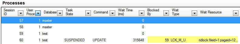
In SSMS, right click on the SQL Server instance name and select Activity Monitor.  In the Processes section you will see information similar to below.  Here we can see similar information as sp_who2, but we can also see the Wait Time, Wait Type and also the resource that SPID 60 is waiting for.

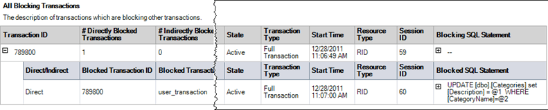
Report - All Blocking Transactions

Another option is to use the built in reports in SSMS.  Right click on the SQL Server instance name and select Reports > Standard Reports > Activity - All Block Transactions.

Querying Dynamic Management Views

You can also use the DMVs to get information about blocking.

SELECT session_id, command, blocking_session_id, wait_type, wait_time, wait_resource, t.TEXT
FROM sys.dm_exec_requests 
CROSS apply sys.dm_exec_sql_text(sql_handle) AS t
WHERE session_id > 50 
AND blocking_session_id > 0
UNION
SELECT session_id, '', '', '', '', '', t.TEXT
FROM sys.dm_exec_connections 
CROSS apply sys.dm_exec_sql_text(most_recent_sql_handle) AS t
WHERE session_id IN (SELECT blocking_session_id 
                    FROM sys.dm_exec_requests 
                    WHERE blocking_session_id > 0)

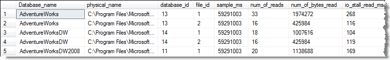
Here is the output and we can see the blocking information along with the TSQL commands that were issued.

Tracing a SQL Server Deadlock    (Performance Issues)

Overview

A common issue with SQL Server is deadlocks.  A deadlock occurs when two or more processes are waiting on the same resource and each process is waiting on the other process to complete before moving forward.  When this situation occurs and there is no way for these processes to resolve the conflict, SQL Server will choose one of processes as the deadlock victim and rollback that process, so the other process or processes can move forward.

By default when this occurs, your application may see or handle the error, but there is nothing that is captured in the SQL Server Error Log or the Windows Event Log to let you know this occurred.  The error message that SQL Server sends back to the client is similar to the following:

Msg 1205, Level 13, State 51, Line 3
Transaction (Process ID xx) was deadlocked on {xxx} resources with another process 
and has been chosen as the deadlock victim. Rerun the transaction. 

In this tutorial we cover what steps you can take to capture deadlock information and some steps you can take to resolve the problem.

Explanation

Deadlock information can be captured in the SQL Server Error Log or by using Profiler / Server Side Trace.

Trace Flags

If you want to capture this information in the SQL Server Error Log you need to enable one or both of these trace flags. 

• 1204 - this provides information about the nodes involved in the deadlock
• 1222 - returns deadlock information in an XML format

You can turn on each of these separately or turn them on together.  

To turn these on you can issue the following commands in a query window or you can add these as startup parameters.  If these are turned on from a query window, the next time SQL Server starts these trace flags will not be active, so if you always want to capture this data the startup parameters is the best option.

DBCC TRACEON (1204, -1)
DBCC TRACEON (1222, -1)

Here is sample output for each of the trace flags.

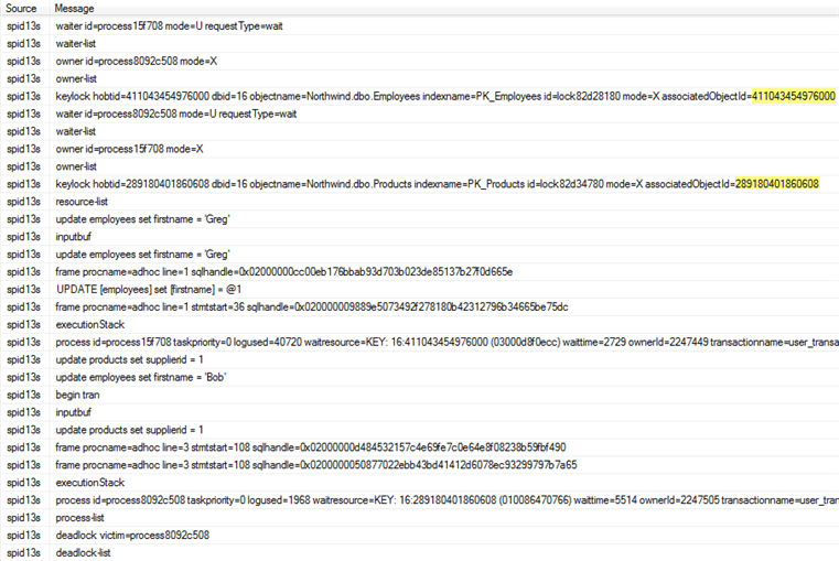
Trace Flag 1222 Output

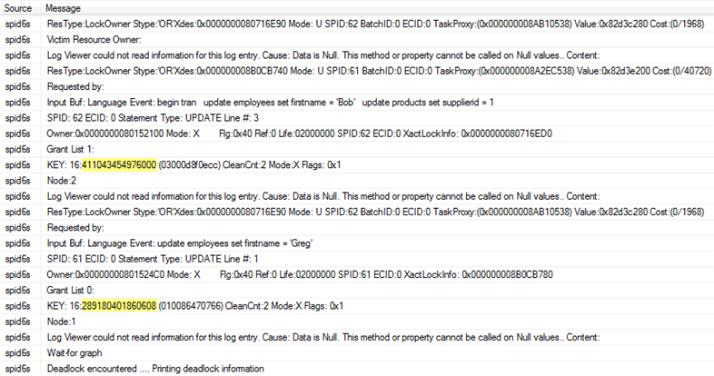
Trace Flag 1204 Output

---

Profiler / Server Side Trace

Profiler works without the trace flags being turned on and there are three events that can be captured for deadlocks.  Each of these events is in the Locks event class.

• Deadlock graph - Occurs simultaneously with the Lock:Deadlock event class. The Deadlock Graph event class provides an XML description of the deadlock.
• Lock: Deadlock - Indicates that two concurrent transactions have deadlocked each other by trying to obtain incompatible locks on resources that the other transaction owns.
• Lock: Deadlock Chain - Is produced for each of the events leading up to the deadlock.

Event Output

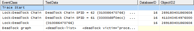
In the below image, I have only captured the three events mentioned above.

Deadlock Graph Output

Below is the deadlock graph which is the output for the Deadlock graph event.  We can see on the left side that server process id 62 was selected as the deadlock victim.  Also, if you hover over the oval with the X through it we can see the transaction that was running.

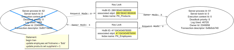
Finding Objects Involved in Deadlock

In all three outputs, I have highlighted the object IDs for the objects that are in contention.  You can use the following query to find the object, substituting the object ID for the partition_id below.

SELECT OBJECT_SCHEMA_NAME([object_id]),
OBJECT_NAME([object_id])
FROM sys.partitions
WHERE partition_id = 289180401860608;

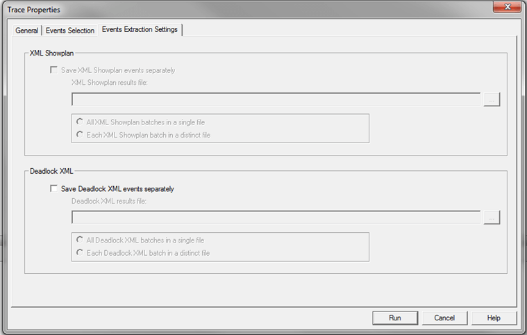
Saving Deadlock Graph Data in XML File

Since the deadlock graph data is stored in an XML format, you can save the XML events separately.  When configuring the Trace Properties click on the Events Extraction Settings and enable this option as shown below.

Index Scans and Table Scans  Overview There are several things that you can do to improve performance by throwing more hardware at the problem, but usually the place you get the most benefit from is when you tune your queries.  One common problem that exists is the lack of indexes or incorrect indexes and therefore SQL Server has to process more data to find the records that meet the queries criteria.  These issues are known as Index Scans and Table Scans. In this section will look at how to find these issues and how to resolve them. Explanation An index scan or table scan is when SQL Server has to scan the data or index pages to find the appropriate records.  A scan is the opposite of a seek, where a seek uses the index to pinpoint the records that are needed to satisfy the query.  The reason you would want to find and fix your scans is because they generally require more I/O and also take longer to process.  This is something you will notice with an application that grows over time.  When it is first released performance is great, but over time as more data is added the index scans take longer and longer to complete. To find these issues you can start by running Profiler or setting up a server side trace and look for statements that have high read values.  Once you have identified the statements then you can look at the query plan to see if there are scans occurring. Here is a simple query that we can run. First use Ctrl+M to turn on the actual execution plan and then execute the query. SELECT * FROM Person.Contact Here we can see that this query is doing a Clustered Index Scan.  Since this table has a clustered index and there is not a WHERE clause SQL Server scans the entire clustered index to return all rows.  So in this example there is nothing that can be done to improve this query.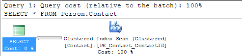 In this next example I created a new copy of the Person.Contact table without a clustered index and then ran the query. SELECT * FROM Person.Contact2 Here we can see that this query is doing a Table Scan, so when a table has a Clustered Index it will do a Clustered Index Scan and when the table does not have a clustered index it will do a Table Scan.  Since this table does not have a clustered index and there is not a WHERE clause SQL Server scans the entire table to return all rows.  So again in this example there is nothing that can be done to improve this query.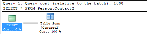 In this next example we include a WHERE clause for the query. SELECT * FROM Person.Contact WHERE LastName = 'Russell' Here we can see that we still get the Clustered Index Scan, but this time SQL Server is letting us know there is a missing index.  If you right click on the query plan and select Missing Index Details you will get a new window with a script to create the missing index.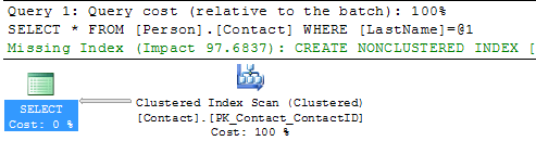 Let's do the same thing for our Person.Contact2 table. SELECT * FROM Person.Contact2 WHERE LastName = 'Russell' We can see that we still have the Table Scan, but SQL Server doesn't offer any suggestions on how to fix this.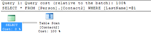 Another thing you could do is use the Database Engine Tuning Advisor to see if it gives you any suggestions. If I select the query in SSMS, right click and select Analyze Query in Database Engine Tuning Advisor the tools starts up and I can select the options and start the analysis. Below is the suggestion this tool provides and we can see that recommends creating a new index, so you can see that using both tools can be beneficial. 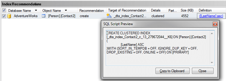Create New Index So let's create the recommended index on Person.Contact and run the query again. USE [AdventureWorks] GO CREATE NONCLUSTERED INDEX [IX_LastName] ON [Person].[Contact] ([LastName]) GO SELECT * FROM Person.Contact WHERE LastName = 'Russell' 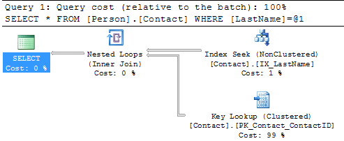Here we can see the query plan has changed and instead of a Clustered Index Scan we now have an Index Seek which is much better.  We can also see that there is now a Key Lookup operation which we will talk about in the next section. Summary By finding and fixing your Index Scans and Table Scans you can drastically improve performance especially for larger tables.  So take the time to identify where your scans may be occurring and create the necessary indexes to solve the problem.  One thing that you should be aware of is that too many indexes also causes issues, so make sure you keep a balance on how many indexes you create for a particular table. Eliminating bookmark (key/rid) lookups Overview When we were looking at the index scan and table scan section we were able to eliminate the scan which was replaced with an index seek, but this also introduced a Key Lookup which is something else you may want to eliminate to improve performance. A key lookup occurs when data is found in a non-clustered index, but additional data is needed from the clustered index to satisfy the query and therefore a lookup occurs.  If the table does not have a clustered index then a RID Lookupoccurs instead. In this section we will look at how to find Key/RID Lookups and ways to eliminate them. Explanation The reason you would want to eliminate Key/RID Lookups is because they require an additional operation to find the data and may also require additional I/O.  I/O is one of the biggest performance hits on a server and any way you can eliminate or reduce I/O is a performance gain. So let's take a look at an example query and the query plan. Before we do this we want to first add the nonclustered index on LastName. USE [AdventureWorks] GO CREATE NONCLUSTERED INDEX [IX_LastName] ON [Person].[Contact] ([LastName]) GO Now we can use Ctrl+M to turn on the actual execution plan and run the select. SELECT * FROM Person.Contact WHERE LastName = 'Russell' If we look at the execution plan we can see that we have an Index Seek using the new index, but we also have a Key Lookup on the clustered index.  The reason for this is that the nonclustered index only contains the LastName column, but since we are doing a SELECT * the query has to get the other columns from the clustered index and therefore we have a Key Lookup.  The other operator we have is the Nested Loops this joins the results from the Index Seek and the Key Lookup. So if we change the query as follows and run this again you can see that the Key Lookup disappears, because the index includes all of the columns. SELECT LastName FROM Person.Contact WHERE LastName = 'Russell' Here we can see that we no longer have a Key Lookup and we also no longer have the Nested Loops operator. If we run both of these queries at the same time in one batch we can see the improvement by removing these two operators. SELECT * FROM Person.Contact WHERE LastName = 'Russell' SELECT LastName FROM Person.Contact WHERE LastName = 'Russell' Below we can see that the first statement takes 99% of the batch and the second statement takes 1%, so this is a big improvement. This should make sense that since the index includes LastName and that is the only column that is being used for both the SELECTed columns and the WHERE clause the index can handle the entire query.  Another thing to be aware of is that if the table has a clustered index we can include the clustered index column or columns as well without doing a Key Lookup. The Person.Contact table has a clustered index on ContactID, so if we include this column in the query we can still do just an Index Seek. SELECT ContactID, LastName FROM Person.Contact WHERE LastName = 'Russell' Here we can see that we only need to do an Index Seek to include both of these columns. So that's great if that is all you need, but what if you need to include other columns such as FirstName. If we change the query as follows then the Key Lookup comes back again. SELECT FirstName, LastName FROM Person.Contact WHERE LastName = 'Russell' Luckily there are a few options to handle this. Creating a Covering Index A covering index basically does what it implies, it covers the query by including all of the columns that are needed.  So if our need is to always include FirstName and LastName we can modify our index as follows to include both LastName and FirstName. DROP INDEX [IX_LastName] ON [Person].[Contact] GO CREATE NONCLUSTERED INDEX [IX_LastName] ON [Person].[Contact] ([LastName], [FirstName]) GO And if we look at the execution plan we can see that we eliminated the Key Lookup once again. Creating an Index with Included Columns Another option is to use the included columns feature for an index.  This allows you to include additional columns so they are stored with the index, but are not part of the index tree.  So this allows you to take advantage of the features of a covering index and reduces storage needs within the index tree. Another benefit is that you can include additional data types that can not be part of a covering index. The syntax for the the index with included columns is as follows: DROP INDEX [IX_LastName] ON [Person].[Contact] GO CREATE NONCLUSTERED INDEX [IX_LastName] ON [Person].[Contact] ([LastName]) INCLUDE ([FirstName]) GO Here we can see the exuection plan is the same for both options. Discovering Unused Indexes Overview To ensure that data access can be as fast as possible, SQL Server like other relational database systems utilizes indexing to find data quickly.  SQL Server has different types of indexes that can be created such as clustered indexes, non-clustered indexes, XML indexes and Full Text indexes. The benefit of having more indexes is that SQL Server can access the data quickly if an appropriate index exists.  The downside to having too many indexes is that SQL Server has to maintain all of these indexes which can slow things down and indexes also require additional storage.  So as you can see indexing can both help and hurt performance. In this section we will focus on how to identify indexes that exist, but are not being used and therefore can be dropped to improve performance and decrease storage requirements. Explanation When SQL Server 2005 was introduced it added Dynamic Management Views (DMVs) that allow you to get additional insight as to what is going on within SQL Server.  One of these areas is the ability to see how indexes are being used.  There are two DMVs that we will discuss.   Note that these views store cumulative data, so when SQL Server is restated the counters go back to zero, so be aware of this when monitoring your index usage. DMV - sys.dm_db_index_operational_stats This DMV allows you to see insert, update and delete information for various aspects for an index.  Basically this shows how much effort was used in maintaining the index based on data changes. If you query the table and return all columns, the output may be confusing.  So the query below focuses on a few key columns.  To learn more about the output for all columns you can check out Books Online. SELECT OBJECT_NAME(A.[OBJECT_ID]) AS [OBJECT NAME], I.[NAME] AS [INDEX NAME], A.LEAF_INSERT_COUNT, A.LEAF_UPDATE_COUNT, A.LEAF_DELETE_COUNT FROM SYS.DM_DB_INDEX_OPERATIONAL_STATS (db_id(),NULL,NULL,NULL ) A INNER JOIN SYS.INDEXES AS I ON I.[OBJECT_ID] = A.[OBJECT_ID] AND I.INDEX_ID = A.INDEX_ID WHERE OBJECTPROPERTY(A.[OBJECT_ID],'IsUserTable') = 1 Below we can see the number of Inserts, Updates and Deletes that occurred for each index, so this shows how much work SQL Server had to do to maintain the index. DMV - sys.dm_db_index_usage_stats This DMV shows you how many times the index was used for user queries.  Again there are several other columns that are returned if you query all columns and you can refer to Books Online for more information. SELECT OBJECT_NAME(S.[OBJECT_ID]) AS [OBJECT NAME], I.[NAME] AS [INDEX NAME], USER_SEEKS, USER_SCANS, USER_LOOKUPS, USER_UPDATES FROM SYS.DM_DB_INDEX_USAGE_STATS AS S INNER JOIN SYS.INDEXES AS I ON I.[OBJECT_ID] = S.[OBJECT_ID] AND I.INDEX_ID = S.INDEX_ID WHERE OBJECTPROPERTY(S.[OBJECT_ID],'IsUserTable') = 1 AND S.database_id = DB_ID() Here we can see seeks, scans, lookups and updates. The seeks refer to how many times an index seek occurred for that index.  A seek is the fastest way to access the data, so this is good. The scans refers to how many times an index scan occurred for that index.  A scan is when multiple rows of data had to be searched to find the data.  Scans are something you want to try to avoid. The lookups refer to how many times the query required data to be pulled from the clustered index or the heap(does not have a clustered index).  Lookups are also something you want to try to avoid. The updates refers to how many times the index was updated due to data changes which should correspond to the first query above. Identifying Unused Indexes So based on the output above you should focus on the output from the second query.  If you see indexes where there are no seeks, scans or lookups, but there are updates this means that SQL Server has not used the index to satisfy a query but still needs to maintain the index.  Remember that the data from these DMVs is reset when SQL Server is restarted, so make sure you have collected data for a long enough period of time to determine which indexes may be good candidates to be dropped. Investigating I/O bottlenecks Overview SQL Server is usually a high I/O activity process and in most cases the database is larger than the amount of memory installed on a computer and therefore SQL Server has to pull data from disk to satisfy queries.  In addition, since the data in databases is constantly changing these changes need to be written to disk.  Another process that can consume a lot of I/O is the TempDB database.  The TempDB database is a temporary working area for SQL Server to do such things as sorting and grouping.  The TempDB database also resides on disk and therefore depending on how many temporary objects are created this database could be busier than your user databases. Since I/O is such an important part of SQL Server performance you need to make sure your disk subsystem is not the bottleneck.  In the old days this was much easier to do, since most servers had local attached storage.  These days most SQL Servers use SAN or NAS storage or to further complicate things more and more SQL Servers are running in a virtualized environment. Explanation There are several different methods that can be used to track I/O performance, but as mentioned above with SAN / NAS storage and virtualized SQL Server environments, this is getting harder and harder to track as well as the rules have changed as far as what should be tracked to determine if there is an I/O bottleneck.  The advantage is that there are several tools available at both the storage level and the virtual level to aid in performance, but we will not cover these here. There are basically two options that you have to monitor I/O bottlenecks, SQL Server DMVs and Performance Monitor counters.  There are other tools as well, but these are two options that will exist in every SQL Server environment. DMV - sys.dm_io_virtual_file_stats This DMV will give you cumulative file stats for each database and each database file including both the data and log files.  Based on this data you can determine which file is the busiest from a read and/or write perspective. The output also includes I/O stall information for reads, writes and total.  The I/O stall is the total time, in milliseconds, that users waited for I/O to be completed on the file.  By looking at the I/O stall information you can see how much time was waiting for I/O to complete and therefore the users were waiting. The data that is returned from this DMV is cumulative data, which means that each time you restart SQL Server the counters are reset.  Since the data is cumulative you can run this once and then run the query again in the future and compare the deltas for the two time periods. If the I/O stalls are high compared to the length of the that time period then you may have an I/O bottleneck. SELECT cast(DB_Name(a.database_id) as varchar) as Database_name, b.physical_name, * FROM sys.dm_io_virtual_file_stats(null, null) a INNER JOIN sys.master_files b ON a.database_id = b.database_id and a.file_id = b.file_id ORDER BY Database_Name Here is partial output from the above command. Performance Monitor Performance Monitor is a Windows tool that let's you capture statistics about SQL Server, memory usage, I/O usage, etc...  This tool can be run interactively using the GUI or you can set it up to collected information behind the scenes which can be reviewed at a later time.  This tool is found in the Control Panel under Administrative tools. There are several counters related to I/O and they are located under Physical Disk and Logical Disk.  The Physical Disk performance object consists of counters that monitor hard or fixed disk drive on a computer.  The Logical Disk performance object consists of counters that monitor logical partitions of a hard or fixed disk drives. For the most part, they both contain the same counters.  In most cases you will probably use the Physical Disk counters.  Here is a partial list of the available counters. Now that storage could be either local, SAN, NAS, etc... these two counters are helpful to see if there is a bottleneck: Avg. Disk sec/Read is the average time, in seconds, of a read of data from the disk. Avg. Disk sec/Write is the average time, in seconds, of a write of data to the disk. The recommendation is that the values for both of these counters be less than 20ms.  When you capture this data the values will be displayed as 0.000, so a value of 0.050 equals 50ms. Resource Monitor Another tool that you can use is the Resource Monitor.  This can be launched from Task Manager or from the Control Panel. Below you can see the Disk tab that shows current processes using disk, the active disk files and storage at the logical and physical level.  The Response Time (ms) is helpful to see how long it is taking to service the I/O request. Additional Information I/O issues may not always be a problem with your disk subsystem.  Just because you see a slow down or I/O waits occurring there may be other issues that you need to consider such as missing indexes, poorly written queries, fragmentation or out of date statistics.  We will cover these topics as well in this tutorial.

Find Keyword in whole Database

T-SQL Script: Find Keyword in whole Database

Ref:

http://www.rad.pasfu.com/index.php?/archives/65-T-SQL-Script-Find-Keyword-in-whole-Database.html#extended

There are some times that you need to find all occurrence (or some of them) of a keyword in all columns/tables in a database, This is a usual scenario in data profiling.

I wrote script below to fulfill this requirement, this script will search for specific keyword in all columns and tables of a database (SQL Server database) and returns list of Schemas, Tables, Columns and occurrence of keyword as a result

declare @keyword nvarchar(max)

set @keyword='David'

declare @schema varchar(max)

declare @table varchar(max)

declare @column varchar(max)

declare @sqlstatement nvarchar(max)

declare @totalrecords int

declare @counter int

declare @occurrence int

declare @objects table

(

SchemaName varchar(max),

TableName varchar(max),

ColumnName varchar(max),

IsProcessed bit,

Occurrence int)

insert into @objects(SchemaName,TableName,ColumnName,IsProcessed)

select sch.name,tab.name,col.name,0

from sys.columns col

inner join sys.tables tab

on col.object_id=tab.object_id

inner join sys.schemas sch

on tab.schema_id=sch.schema_id

where col.system_type_id not in (

34,--image

241--xml

)

order by sch.name,tab.name,col.name

select @totalrecords=count(*) from @objects

set @counter=0

while (@counter<=@totalrecords)

begin

select top 1 @schema=SchemaName,@table=TableName,@column=ColumnName

from @objects

where isprocessed=0

order by SchemaName,TableName,ColumnName

set @sqlstatement='select @occurrence=count(*) from ['+@schema+'].['+@table+'] where ['+@column+'] like ''%'+@keyword+'%'''

exec sp_executesql @query=@sqlstatement,@params=N'@occurrence int output',@occurrence=@occurrence output

update @objects

set IsProcessed=1,

Occurrence=@occurrence

where SchemaName=@schema and TableName=@table and ColumnName=@column

set @counter=@counter+1

end

select SchemaName,TableName,ColumnName,Occurrence from @objects

This script took 5 minutes to run on a database with 120 tables (total number of 1400 columns)

This is sample result of script:

To run this script you just need to open a query window in SSMS, select database, change value assigned to @keyword variable and run the query.

To Make Source and Destination Table Same in SSIS

Make Source and Destination Table Same in SSIS

Insert, Update, and Delete Destination table with SSIS

Ref:

http://www.rad.pasfu.com/index.php?/archives/150-Insert,-Update,-and-Delete-Destination-table-with-SSIS.html

Previously I’ve wrote about design and implementation an UPSERT with SSIS. UPSERT is about Update existing records, and Insert new records. Today I want to extend this to cover DELETED records as well. So method used in this post can be used to find INSERTED / UPDATED / DELETED records from the source table and apply those changes into the destination table.

In this example I used Merge Join Transformation, Conditional Split, and OLE DB Command transform to implement the solution. First we apply a full outer join on source and destination table on key column(s) with Merge Join transformation. Then we use a conditional split to find out the change type (removed, new, or existing records). Existing records will require another processing to find out is there any changes happened or not? We use another conditional split to compare value of equivalent columns in source and destination.

Source table used in this example is Department table from AdventureWorks2012 sample database which you can download online for free.

Solution:

1- Create an OLE DB Source for source table, use select command below to select data:

select *

from dbo.Department

order by DepartmentID

Note to the ORDER BY Clause in this statement. That part is required because Merge Join transform require sorted sources as input. Name this component as Source Table

2- Create another OLE DB Source for destination table. In this example source and destination has same table name but are in different databases. So we use same script as step 1 for this one as well. Name this component as Destination Table.

3- Right click on OLE DB Source, choose Show Advanced Editor. In the Advanced Editor window go to Input and Output Properties tab. Select the OLE DB Source Output, and change the IsSorted Property to true.

4- Expand OLE DB Source output, and then under Output Columns select DepartmentID. Then change the SortKeyPosition to 1.

5- Apply steps 3 and 4 for both OLE DB Sources (Source Table and Destination Table)

6- Drag and drop a Merge Join transformation, connect two OLE DB Sources to this. Set Source Table as left and Destination Table as right input of this transformation.

7- Go to Merge Join transformation editor, DepartmentID will be used as joining column (selected based on sort properties of previous components). Note that if you don’t sort input columns of the merge join transformation then you cannot get into the editor of this transformation and you face the error regarding sorting of inputs.

Select all columns from Source and Destination tables in the merge join transform, and rename them as picture below shows (add Source or Destination prefix to each column)

8- Add a Conditional Split transformation and write two expressions below to find out new records, and removed records. Also rename default output as existing records and screenshot below shows

Expressions used in this sample are very easy and simply find record changes. For example expression below:

!ISNULL(SourceDepartmentID) && ISNULL(DestinationDepartmentID)

Used to find new records. And literally means records that has SourceDepartmentID but not DestinationDepartmentID.

And this script used to find deleted records:

ISNULL(SourceDepartmentID) && !ISNULL(DestinationDepartmentID)

9- Add an OLE DB Destination and connect NEW RECORDS output to it. Set configuration for destination table and use columns with Source prefix in the column mapping of the OLE DB destination. This destination component will insert new records into the destination table.

10- Add an OLE DB Command and connect Removed RECORDS output to it. Create a connection to destination database, and write script below to delete records by input department ID:

delete from dbo.department where DepartmentID=?

In the column mappings, map DestinationDepartmentID to the parameter of statement.

11- Add another Conditional Split and connect Existing Records output to it. We use this component to find only records that had a change in one of the values. So we compare equivalent source and destination columns to find non-match data.

This is the expression used to find match data in screenshot below:

(SourceName == DestinationName) && (SourceGroupName == DestinationGroupName) && (SourceModifiedDate == DestinaitonModifiedDate)

12- Create a stored procedure in destination database to update the Department table.

CREATE PROCEDURE dbo.UpdateDepartment

@DepartmentID smallint

,@Name nvarchar(50)

,@GroupName nvarchar(50)

,@ModifiedDate datetime

AS

BEGIN

SET NOCOUNT ON;

UPDATE [dbo].[Department]

SET

[Name] = @Name

,[GroupName] = @GroupName

,[ModifiedDate] = @ModifiedDate

WHERE [DepartmentID] = @DepartmentID

END

13- Add another OLE DB Command and use non match output as the input data stream to it. Connect it to destination database, and write below statement in Component Properties tab’s SQLCommand property.

exec dbo.UpdateDepartment ?,?,?,?

14- Map input columns (with source prefixes) to parameters in the stored procedure as screenshot below shows

15- Run the package and you will see changes will be applied to destination table.

Testing the solution:

Here is data rows from source table

And data rows from destination table

Yellow records are new records

Pink records are updated records

Green record is deleted record (in destination table)

After running the package you will see records will be redirected to data path as implemented:

And destination table will pick changes:

Posted by Reza Rad on Tuesday, September 10. 2013 at 20:2

Types of Joins in SQL Server

A Visual Explanation of SQL Joins

Ref: http://blog.codinghorror.com/a-visual-explanation-of-sql-joins/

INNER JOIN
FULL OUTER JOIN
LEFT OUTER JOIN
RIGHT OUTER JOIN
CROSS JOIN

Assume we have the following two tables. Table A is on the left, and Table B is on the right. We'll populate them with four records each.

id name       id  name
-- ----       --  ----
1  Pirate     1   Rutabaga
2  Monkey     2   Pirate
3  Ninja      3   Darth Vader
4  Spaghetti  4   Ninja

Let's join these tables by the name field in a few different ways and see if we can get a conceptual match to those nifty Venn diagrams.

SELECT * FROM TableA INNER JOIN TableB ON TableA.name = TableB.name id name id name -- ---- -- ---- 1 Pirate 2 Pirate 3 Ninja 4 Ninja Inner join produces only the set of records that match in both Table A and Table B.
SELECT * FROM TableA FULL OUTER JOIN TableB ON TableA.name = TableB.name id name id name -- ---- -- ---- 1 Pirate 2 Pirate 2 Monkey null null 3 Ninja 4 Ninja 4 Spaghetti null null null null 1 Rutabaga null null 3 Darth Vader Full outer join produces the set of all records in Table A and Table B, with matching records from both sides where available. If there is no match, the missing side will contain null.
SELECT * FROM TableA LEFT OUTER JOIN TableB ON TableA.name = TableB.name id name id name -- ---- -- ---- 1 Pirate 2 Pirate 2 Monkey null null 3 Ninja 4 Ninja 4 Spaghetti null null Left outer join produces a complete set of records from Table A, with the matching records (where available) in Table B. If there is no match, the right side will contain null.
SELECT * FROM TableA LEFT OUTER JOIN TableB ON TableA.name = TableB.name WHERE TableB.id IS null id name id name -- ---- -- ---- 2 Monkey null null 4 Spaghetti null null To produce the set of records only in Table A, but not in Table B, we perform the same left outer join, then exclude the records we don't want from the right side via a where clause.
SELECT * FROM TableA FULL OUTER JOIN TableB ON TableA.name = TableB.name WHERE TableA.id IS null OR TableB.id IS null id name id name -- ---- -- ---- 2 Monkey null null 4 Spaghetti null null null null 1 Rutabaga null null 3 Darth Vader To produce the set of records unique to Table A and Table B, we perform the same full outer join, then exclude the records we don't want from both sides via a where clause.

There's also a cartesian product or cross join, which as far as I can tell, can't be expressed as a Venn diagram:

SELECT * FROM TableA
CROSS JOIN TableB

This joins "everything to everything", resulting in 4 x 4 = 16 rows, far more than we had in the original sets. If you do the math, you can see why this is a very dangerous join to run against large tables.
QUIZ:
This Question was asked by interview.
Any one Can answer this question BY comment this blog?
 Write Query B shaded Area?

Ans:

SELECT * FROM TableA 

RIGHT OUTER JOIN TableB 

ON TableA.name = TableB.name 

WHERE TableA.id IS null

O/P:

ID     Name

1 Rutabaga

3 Darth Vader

Definition Of Joins:

1. Left Outer Join.
2. Right Outer Join.
3. Full Outer Join.

Left Outer Join - A Left Outer Join in SQL Server returns the “Matched Rows”  from multiple tables and “Non Matched Rows” from Left side table. Follow the above picture for more understanding.

Right Outer Join - A Right Outer Join in SQL Server returns the “Matched Rows” from multiple tables and“Non Matched Rows” from Right side table. Follow the above picture for more understanding.

Full Outer Join - A Full Outer Join returns “Matched Rows” from multiple tables and also “Non Matched Rows” from multiple tables. Follow the above picture for more understanding.

Difference between Row_Number, Rank, Dense_Rank Functions

Difference between Row_Number, Rank, Dense_Rank

Difference between Row_Number, Rank, Dense_Rank

Syntax and use:

Row_Number 

Returns the sequential number of a row within a partition of a result set, starting at 1 for the first row in each partition.

ROW_NUMBER ( )     OVER ([<partition_by_clause>] <order_by_clause>)

Rank 
Returns the rank of each row within the partition of a result set. The rank of a row is one plus the number of ranks that come before the row in question.

RANK ( )    OVER ([< partition_by_clause >] < order_by_clause >)

Dense_Rank

 Returns the rank of rows within the partition of a result set, without any gaps in the ranking. The rank of a row is one plus the number of distinct ranks that come before the row in question.

DENSE_RANK ( )    OVER ([<partition_by_clause> ] < order_by_clause > )

NTILE 

Distributes the rows in an ordered partition into a specified number of groups. The groups are numbered, starting at one. For each row, NTILE returns the number of the group to which the row belongs.

NTILE (integer_expression) OVER ([<partition_by_clause>] < order_by_clause >)

Where

<partition_by_clause>

Divides the result set produced by the From clause into partitions to which the Row_Number/ Rank/ Dense_Rank/ Ntile function is applied.

<order_by_clause>

Determines the order in which the Row_Number/ Rank/ Dense_Rank/ Ntile values are applied to the rows in a partition. 

We will apply these function on the below customer product table CustProd.

name	Product
cust1	decoder
cust2	cable
cust1	cable
cust2	package
cust3	decoder
cust3	cable

Please see the below snapshot for understanding of these function through example

With partition by product and order by name,

When we use partition by product, then it divides the result on the basis of product, as there are three distinct products then there will be 3 partitions.

After partition, order by name is used, that means, in the partitions Row Number, Rank or Dense Rank will be assigned as per the order of name. Here in the below result we see that rank ,row number and dense rank, all are having same value, It’s because in each partition there are distinct name given, if name would have been repeated for the same product then those records will have same rank and dense rank, but row number would have been same as shown below.

When used order by product instead of name , then we see in the below result that, the Rank and dense Rank were 1, Because we did partition of result by product , that means there will be common product in each partition , and rank and dense rank will also be same for same product.